7/1 Nonlinear Function Approximation with Multilayer Perceptrons
Note that in all supervised learning tasks so far, we were optimizing affine transformations
Synthetic Dataset: Hypersphere Classification
Let us introduce a synthetic classification dataset that logistic regression may not be able to handle: the feature vectors of a given class \(c\in[C]\) are sampled from the distribution
$$ r_c\left(\mathscr U(S^{n-1})+\mathscr N(\mathbf0,s)\right)+\mathbf x_c, $$ that is:
-
We sample points from the uniform distribution on an \((n-1)\)-dimensional hypersphere
\[ S^{n-1}=\{(x_1,\dotsc,x_n)\in\mathbf R^n:x_1^2+\dotsb+x_n^2=1\}, \] -
we add additive noise to this, sampled from the normal distribution with mean 0 and std \(s\),
- we multiply the sum with the radius \(r_c\in\mathbf R_{>0}\)
- and finally we translate the product with the offset \(\mathbf x_c\in\mathbf R^n\).
For example, here's how 10 000 samples from the datasets with
- the same number of classes \(C=2\),
- the same ambient dimension \(n=2\),
- the same radii \(0.8, 1.2\)
- the same additive noise std \(0.1\),
- the same negative offset \((0, 0)\) and
- varying positive offsets \((0, 0), (1, 1), (4, -2)\)
look like:
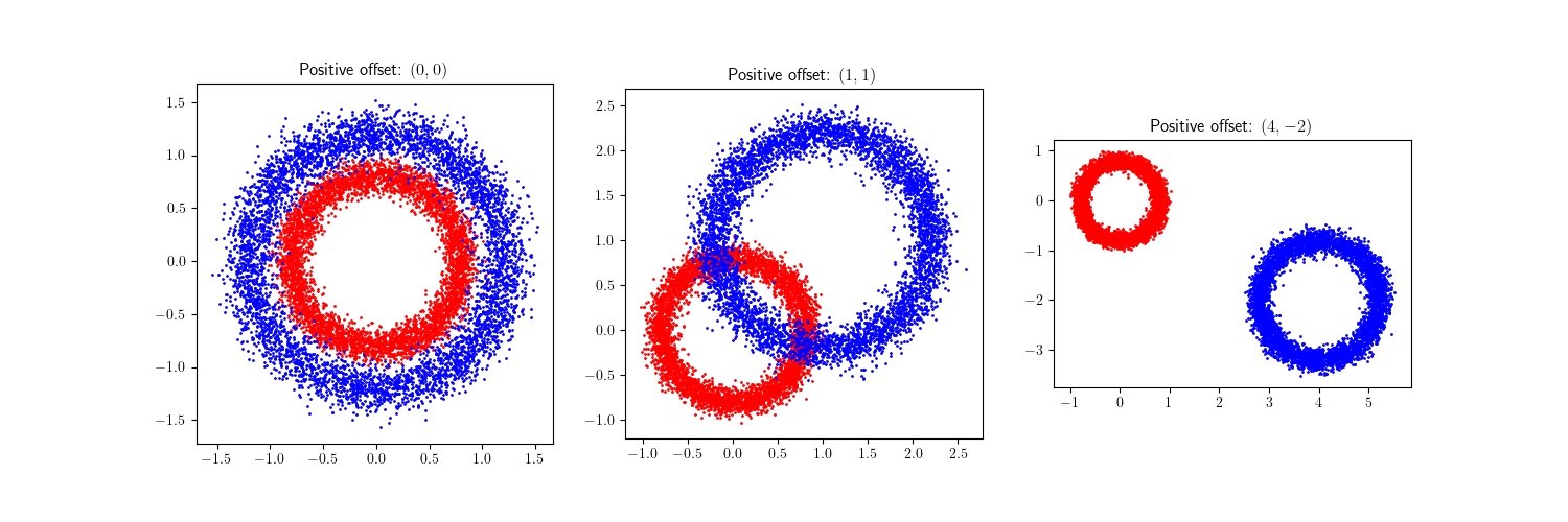
Synthetic classification datasets with \(n=2\) feature dimensions. The colors of the vertices signify the classes of the dataset entries.
Binary Classification
In case \(C=2\), the task is binary classification. This can be handled in a special way, making it simpler than the more general, multiclass case.
Bernoulli Distribution
Recall that for classification problems with \(C\) possible outcomes, we used categorical distribution \((p_0,\dotsc,p_{C-1})\). In case \(C=2\), we get \(p_1 = 1 - p_0\). We see that it is enough to calculate \(p_0\).
It is customary to name the two outcomes the negative and positive outcomes and use the Bernoulli distribution as model, where there is only one parameter: the probability \(p\) of the positive outcome.
Sigmoid and Logit Functions
So, our affine transformation will have 1-dimensional output. We'll transform this real number to a probability with the sigmoid (logistic) function $$ p=\sigma(z)=\frac{1}{1-e^{-z}}. $$ The inverse of this function is the logit function $$ z=\log\frac{p}{1-p}. $$ Its values, the logits, stand for logistic units.
Binary Accuracy
Note that to calculate accuracy, we need to transform the probability to a prediction. Usually, we say the model predicts an entry positive, if the probability is larger than 50%. Note the following:
- This agrees with the multiclass case: \(p>1-p\) if and only if \(p>1/2\).
- It is equivalent to ask if the logit is positive.
Binary Cross-Entropy
We need to make a similar change to cross-entropy. Let us use 0 as the negative and 1 as the positive label. Then we can calculate cross-entropy as $$ \ell(\mathbf x, y; \theta)=y\log(\sigma(p_\theta(\mathbf x)))+(1-y)\log(1-\sigma(p_\theta(\mathbf x))) $$
Decision Boundary
Note that for a binary logistic regression classifier
$$ \mathbf P_\theta(Y=1|X=\mathbf x)=\sigma(\mathbf x^T\mathbf w+b), $$ the model predicts \(\mathbf x\) is positive if this probability is larger that 50%, which is equivalent to
$$ \mathbf x^T\mathbf w+b>0. $$ Therefore, the entries that are predicted positive and negative are separated by the hyperplane
$$ \mathbf x^T\mathbf w+b=0, $$ the so-called decision boundary.
We'll train logistic regression classifiers by SGD on the synthetic datasets. For now, I'll write the accuracies, and draw the decision boundaries:
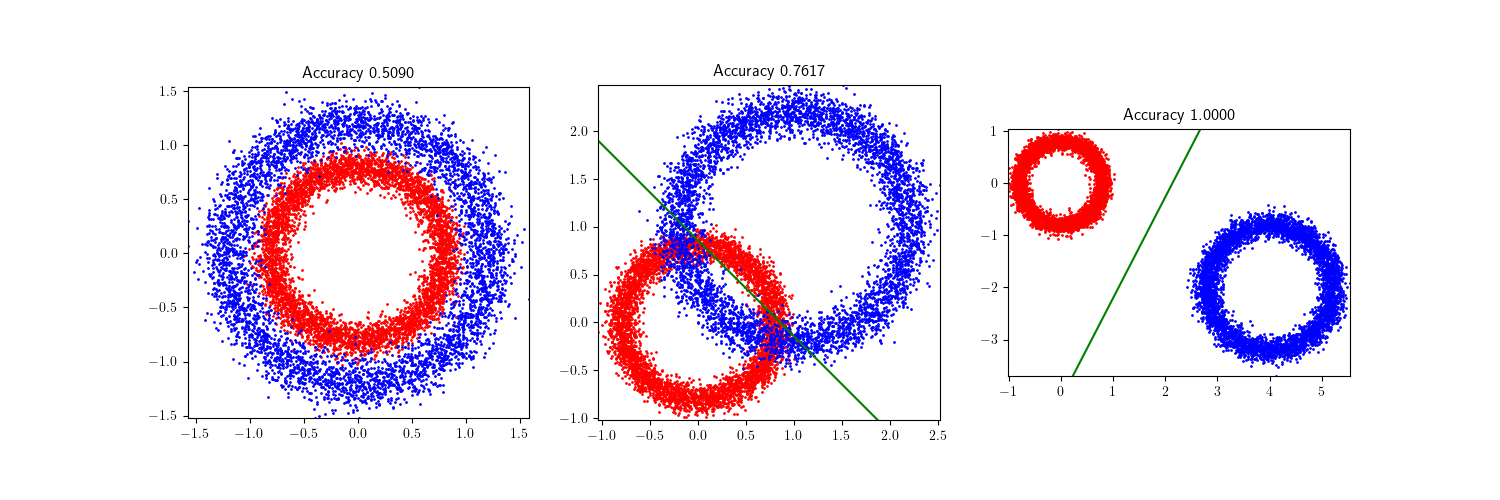
Logistic regression on the synthetic datasets. The lines are the decision boundaries.
Question
Why can't we see the decision boundary in the left-hand case of no positive class offset?
Perceptrons
Given a binary logistic regression model $$ \mathbf x\mapsto\mathbf P_\theta(Y=1:X=\mathbf x)=\sigma(\mathbf x^T\mathbf w+b), $$ we can get the predicted class model as $$ \mathbf x\mapsto H(\mathbf x^T\mathbf w+b), $$ where \(H\) is the Heaviside step (threshold) function1
We call the predicted class model a perceptron.
Piecewise linear decision boundary with ReLU
Consider the 1D hypersphere dataset with no offset:

Synthetic dataset with \(n=1\) feature dimension and no positive class offset.
Just like in the 2D case, there is no linear classifier that can succesfully separate the two classes. On the other hand, if we are allowed piecewise linear decision boundaries, we can do this:
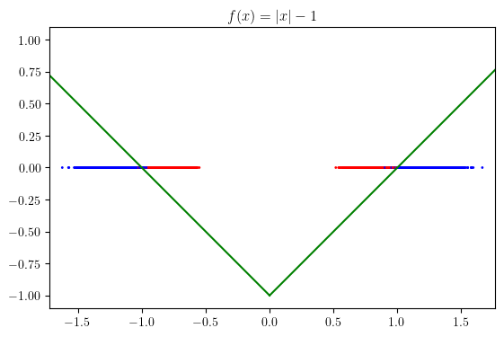
Graph of the piecewise linear decision boundary.
It turns out that we can get a decision boundary like this with an Artificial Neural Network. We'll see in the universal approximation theorem that we only need to use one non-polynomial scalar-to-scalar function. A common choice is the Rectified Linear Unit (ReLU), that sets negative values to 0 elementwise:
With this, we can form our binary classifier as
Let's see what this function does one operation at a time!
Here's the dataset again:
Synthetic 1-dimensional dataset with no positive class offset.
First of all, it applies the linear transformation \(x \mapsto x\cdot\begin{pmatrix} 1 \\ -1 \end{pmatrix}\)
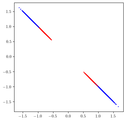
The dataset transformed by \(x \mapsto x\cdot\begin{pmatrix} 1 & -1 \end{pmatrix}\)
Then it applies ReLU elementwise
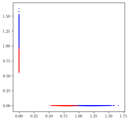
The dataset transformed by \(x \mapsto \mathrm{ReLU}\left(x\cdot\begin{pmatrix} 1 & -1 \end{pmatrix}\right)\)
Finally, it applies the linear transformation \(\mathbf h\mapsto \mathbf h^T\cdot \begin{pmatrix} 1 \\ 1 \end{pmatrix} - 1\). Instead of plotting the 1D image, we plot the previous image together with the decision boundary we get with this.
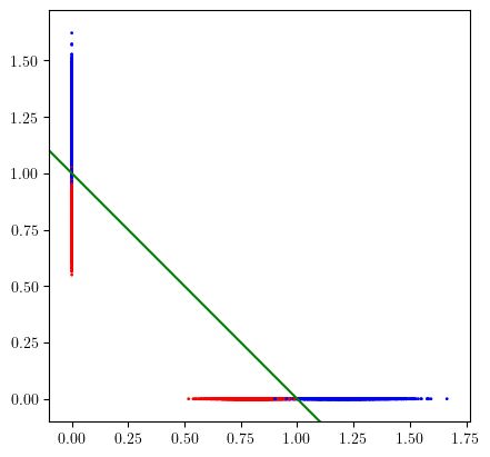
The dataset transformed by \(x \mapsto \mathrm{ReLU}\left(x\cdot\begin{pmatrix} 1 & -1 \end{pmatrix}\right)\), together with the decision boundary of the function \(\mathbf h\mapsto \mathbf h^T\cdot \begin{pmatrix} 1 \\ 1 \end{pmatrix} - 1\)
We get an accuracy rate of about 97.3%. Note that the function \(x \mapsto \mathrm{ReLU}\left(x\cdot\begin{pmatrix} 1 & -1 \end{pmatrix}\right)\) transformed the feature vectors in a way that using an affine classifier \(\mathbf h\mapsto \mathbf h^T\cdot \begin{pmatrix} 1 \\ 1 \end{pmatrix} - 1\) became feasible.
-
The value of \(H(0)\) changes by convention. ↩