6/16 Linear Regression
Today, we'll go through the "Hello World" of machine learning: linear regression on a small dataset.
Course Logistics: Homework
You will get assigned homework roughly twice per week. Each homework will be due 1 week after the day it was announced, at 10:00 am. A precise schedule will be provided. You can expect me to answer a question related to a homework if asked at least 24 hours prior to this time.
Time-Based Multiplier
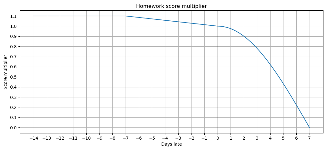
If you hand in your homework earlier than the deadline, you get a bonus, and if you hand it in at most 3 days late, you can still get some score for it, although with a penalty multiplier. The precise formula is as follows: let \(t\) denote the number of days you handed in your homework late. Then your homework score is going to be multiplied by
- \(1.1\), if \(t<-3\),
- \(1.1 - \frac{t + 3}{30}\), if \(-3\le t<0\),
- \(\cos\left(\frac{t}{3}\cdot\frac{\pi}{2}\right)\), if \(0\le t<3\), and
- \(0\), if \(3\le t\).
That is, for example:
- If you hand in your homework 3 days early, your score will be multiplied by \(1.1\).
- If you hand in your homework 2 days early, your score will be multiplied by \(1 + \frac{2}{30}\approx1.067\).
- If you hand in your homework 1 day early, your score will be multiplied by \(1 + \frac{1}{30}\approx1.033\).
- If you hand in your homework 3 hours late, your score will be multiplied by \(\cos\left(\frac{3}{24\cdot3}\cdot\frac{\pi}{2}\right)\approx0.998\).
- If you hand in your homework 12 hours late, your score will be multiplied by \(\cos\left(\frac{12}{24\cdot3}\cdot\frac{\pi}{2}\right)\approx0.966\).
- If you hand in your homework 1 day late, your score will be multiplied by \(\cos\left(\frac{1}{3}\cdot\frac{\pi}{2}\right)\approx0.866\).
- If you hand in your homework 2 days late, your score will be multiplied by \(\cos\left(\frac{2}{3}\cdot\frac{\pi}{2}\right)\approx0.500\).
Your worst homework score will be dropped.
Early Grading Requests
Since homeworks are due 1 week after they were announced, and they have a nonzero multiplier up to 3 days after the deadline, by default, I will start grading homeworks 10 days after they were announced. If you would like to have your homework graded earlier, you can write me an email where you state that:
- your most recent submission is final, and
- you will not discuss the feedback you received with any of your classmates until 3 days after the deadline,
and then I will try to grade your homework earlier.
Hand-In Instructions
Please hand in homework via email, in py files. The filename should have the pattern {name}-{homework id}.py. For example, I would submit the third homework as pal-zsamboki-3.py. If you import from a custom file, please include that in your submission too.
Please make sure that your homework file can be run as intended, using
python {name}-{homework id}.py
- Safest: Copy the full
pyfile contents to a single cell in a new notebook, and run it. - Less safe, but faster: Perform Reset and Run All on the notebook. This helps make sure that all variables are defined explicitly in the notebook.
In either case, if you can only test your submission in notebook format, make sure that you delete notebook-only commands such as
- Terminal commands starting with
!or - Magic commands starting with
%.
Collaboration and External Sources
You are strongly encouraged to discuss homework problems with other students in the course, however, you are required to write your own solutions. You are supposed to understand your own solutions in full detail.
If you rely on sources different from the course notes, it is expected that you name these sources and the extent you have made use of them. In particular, if you rely on a AI assistant (chatbot), please indicate the model name (eg. ChatGPT 5.5 or Gemini 3.5 Flash).
Setup: Regression
Let's recall the task setup from last time. We are given the following objects:
- The (input) feature space, that for now will be the subset of a Euclidean space \(\mathscr X\subseteq\mathbf R^d\). This is the set of outcomes for the input feature random variable \(\mathbf X\).
- The target space, that in case of regression is also a subset of a Euclidean space \(\mathscr Y\subseteq\mathbf R^k\). This is the set of outcomes for the target random variable \(\mathbf Y\).
- A dataset
$$ \mathscr D=\{(\mathbf x_i, \mathbf y_i)\in\mathscr X\times\mathscr Y:i\in I\}, $$ a collection of samples from the joint distribution \((\mathbf X,\mathbf Y)\). Let \(N=|\mathscr D|\).
Stack Vectors in Dataset
Since for each dataset entry index \(i\in I\), the input features \(\mathbf x_i\) and the targets \(y_i\) are both vectors, we can stack them. Thus, we create the input feature and target matrices \(X\in\mathbf R^{N\times d}\), \(Y\in\mathbf R^{N\times k}\) such that for each \(i\in I\), the \(i\)-th row of \(X\) is \(\mathbf x_i\), and the \(i\)-th row of \(Y\) is \(\mathbf y_i\).
Warning
Note that this means feature and target vectors will be represented as row vectors in the dataset.
- This is usual in machine learning (ML) as data traditionally comes in a table, where rows correspond to data entries, and columns correspond to features.
- Moreover, it will be more convenient to perform computations on multiple data entries like this.
- As this is unusual for Mathematicians, in formulas, vectors will be thought of as column vectors. I'll transpose them to make them row vectors.
In case \(k=1\) we drop the target feature dimension from notation: the targets \(y_i\) will be scalars and we'll stack them to a target vector \(\mathbf y\in\mathbf R^N\).
Dataset: Abalone
We'll use the Abalone dataset. In this dataset, we're trying to predict the age of abalone through 8 other measurements such as sex or length.
Preprocessing: One-Hot Encoding
Out of the 8 measurements, we have 7 scalar features. On the other hand, sex is a categorical feature with 3 possible values: female, infant and male. Therefore, the feature space is a subset of the product \(\mathbf R^7\times\{F, I, M\}\).
To be able to use linear regression, we need to convert this feature space to a subset of a Euclidean space. This is part of preprocessing: that is how we call the transformations we perform on the dataset prior to training.
The canonical way to transform categorical features to feature vectors is one-hot encoding: given a finite set \(C=\{c_0,\dotsc,c_{l-1}\}\), we map entry \(c_j\) to the \(j\)-th standard unit vector \(e_j\in\mathbf R^l\).
With this, we get an input feature space with \(d=10\) dimensions.
Model: Affine Transformation
Our model will be an affine transformation $$ f(\mathbf x;\theta)=\mathbf x^T\cdot\mathbf w + b $$ where \(\mathbf w\in\mathbf R^{d}\) is the weight vector and \(b\in\mathbf R\) is the bias. That is, we have \(d':=d+1\) parameters: \(\theta'=(\mathbf w, b)\).
Preprocessing: Add Contant 1 Feature
To simplify notation, we can augment the feature vectors \(\mathbf x\) with a constant 1 feature: for a feature vector \(\mathbf x\in\mathbf R^d\), let \(\tilde{\mathbf x}=(\mathbf x,1)\in\mathbf R^{d'}\). Then we can formulate our model as a linear transformation: $$ f(\mathbf x; \theta')=\tilde{\mathbf x}^T\cdot\mathbf w' $$ where the weight vector \(\mathbf w'=(\mathbf w, b)\).
Question
In this particular case, do we actually need this constant 1 feature? Or is it redundant (linearly dependent on the other features)?
Loss: Mean Squared Error
Having decided on the model \(f_\theta\), we need to decide which parameter vector \(\theta\in\mathbf R^d\) to use. The conventional approach in ML is to use a loss function that, given a parameter vector \(\theta\) and a dataset entry \((\mathbf x_i,y_i)\), outputs an error value \(\ell(x_i,y_i;\theta)\in\mathbf R\). In case of regression an often used loss function is Squared Error (SE): $$ \ell_{SE}(\mathbf x_i,y_i;\theta)=|f_\theta(\mathbf x_i)-y_i|^2. $$
To get overall performance on the dataset, we can take the average $$ \ell(\mathscr D;\theta)=\frac{1}{N}\sum_{i\in I}\ell(\mathbf x_i,y_i;\theta) $$ of the losses on the dataset entries.
In case of SE, we get as dataset-level loss function Mean Squared Error (MSE) $$ \ell_{MSE}(\mathscr D;\theta)=\frac{1}{N}\sum_{i\in I}\ell_{SE}(x_i,y_i;\theta). $$
Preprocessing: Train-Test Split
Recall that we think of the dataset \(\mathscr D\) as a sample from the joint distribution of \(X\) and \(Y\). Therefore, we need \(f_\theta\) to generalize to unseen data. That is, what we actually want to minimize is the expected loss $$ \mathbf E\ell(X, Y;\theta). $$ Now we can't actually compute this, that's why we estimate it with the average loss on a dataset.
This means that we need two datasets, sampled independently: a train dataset \(\mathscr D_\text{train}\sim(X, Y)\) and a test dataset \(\mathscr D_\text{test}\sim(X, Y)\). With this, we
- Set \(\theta\) so that \(\ell(\mathscr D_\text{train}; \theta)\) is small (we can't necessarly find the global minimum, but we try).
- Calculate \(\ell(\mathscr D_\text{test}; \theta)\) with the same \(\theta\). This estimates how well our model \(f_\theta\) generalizes to unseen data.
Often we only have access to a single dataset \(\mathscr D=((x_i, y_i): i\in I)\). In this case, we perform a train-test split:
- We decide on a train-test proportion. Usually this is 85%-15% or 90%-10%. Let's denote these by \(p_\text{train}\) and \(p_\text{test}\).
- We randomly separate the index set \(I\) to a \(p_\text{train}\) portion \(I_\text{train}\) and a \(p_\text{test}\) portion \(I_\text{test}\) (with rounding).
- We let \(\mathscr D_\text{train}=((x_i, y_i): i\in I_\text{train})\) and \(\mathscr D_\text{test}=((x_i, y_i): i\in I_\text{test})\).
In the case of Abalone, the entire dataset \(\mathscr D\) has 4177 entries. With a 85%-15% train-test split, we'll get a train set \(\mathscr D_\text{train}\) of 3550 entries and a test set \(\mathscr D_\text{test}\) of 627 entries.
Preprocessing: Summary
To summarize, we perform the following operations on the dataset:
- Using one-hot encoding, we transform the categorical features to numerical vectors.
- In general, we may add an additional constant 1 feature so that the model can be written as a linear transformation. But in this case, that would be redundant, we can use a linear transformation without the extra feature.
- As we have only one dataset, we make a train-test split.
- To simplify notation, we stack the feature vectors to a feature matrix and the targets to a target vector.
We ended up with the following data:
- a \(3550\times10\) train feature matrix \(X_\text{train}\),
- a 3550-dimensional train target vector \(\mathbf y_\text{train}\),
- a \(627\times10\) test feature matrix \(X_\text{test}\) and
- a 627-dimensional test target vector \(\mathbf y_\text{test}\),
Training: Least Squares
After scalar multiplication, we are trying to find the minimum of the cumulated loss $$ \ell(\mathbf w)=|X_\text{train}\mathbf w - \mathbf y_\text{train}|^2 $$ That is, we're solving a least squares problem. As you may have seen this in a course and we don't actually need the solution method, I describe it in an appendix below.
In the coding portion, we just need two things:
- Check that the columns of \(X\) are independent and if not, discard redundant columns. That is, we want no redundant features.
- Use the built-in least squares solver of
torch.
Note that this is the only problem in this course where we can actually find the global minimum of the function we're trying to optimize. In case of the problems to come, we'll only be able to approximate the minimum.
Appendix: Least Squares
We are trying to find the minimum of the cumulated loss $$ \ell(\mathbf w)=|X\mathbf w - \mathbf y|^2 $$ Up to discarding redundant columns, we can assume that the columns of \(X\) are independent.
Our treatment of least squares follows the textbook Murphy - Probabilistic Machine Learning: An Introduction, Subsection 11.2.2.
Use Dot Product Rules
Recall that
- The squared length \(|\mathbf v|^2\) of a vector is the dot product \(\mathbf v^T\cdot\mathbf v\).
- The dot product \((\mathbf v, \mathbf w)\mapsto\mathbf v^T\cdot\mathbf w\) is a symmetric, bilinear operation.
With this, we can rewrite our cumulated loss as
Calculate gradient
Our cumulated loss function is a vector-to-scalar function \(\mathbf R^d\xrightarrow\ell\mathbf R\). The local extrema (minima and maxima) of such a function are among the vanishing points of its gradient. The gradient is the vector-to-vector function $$ \nabla_\mathbf w\ell=\left(\frac{\partial\ell}{\partial w_1},\dotsc,\frac{\partial\ell}{\partial w_d}\right) $$
To calculate the gradient of our particular function, we can use the identity $$ \nabla_\mathbf x(\mathbf x^TA\mathbf x)=(A+A^T)\mathbf x. $$
With this, we get $$ \nabla_\mathbf w\ell=2X^TX\mathbf w-2X^T\mathbf y. $$
Solve normal equation
That is, a parameter vector \(\mathbf w\) is a local extremum of \(\ell\) if and only if we have $$ X^TX\mathbf w=X^T\mathbf y. $$ This is called the normal equation of the system: geometrically, the solution \(\mathbf w\) is the orthogonal projection of \(\mathbf y\) onto the subspace generated by the rows of \(X\).
As the columns of \(X\) are independent, the matrix \(X^TX\) is invertible, thus the normal equation has a unique solution.
Note that Mathematically, we can write the solution as $$ \mathbf w=(X^TX)^{-1}X^T\mathbf y. $$ But on a computer, this would be wasteful. Instead, we use the least squares solver functionality directly.
Calculate Hessian
We found out that there is a unique vanishing point of the gradient \(\nabla_\mathbf w\ell\). To see if this is an extremum of \(\ell\), we can calculate the Hessian, that is the matrix
In this particular case, we have $$ H(\ell)=X^TX. $$
This matrix is positive definite: for all \(\boldsymbol0\ne\mathbf v\in\mathbf R^d\), as the columns of \(X\) are linearly independent, we have $$ \mathbf v^TX^TX\mathbf v=|X\mathbf v|^2>0. $$
This shows that the function \(\ell\) is convex, thus the unique vanishing point \(\mathbf w\) of \(\nabla_\mathbf w\ell\) we found is the global minimum.